Downloading and Processing CERRA Climate Data from CDS

Introduction

This document outlines a complete workflow to download and process CERRA reanalysis climate data from the Copernicus Climate Data Store (CDS). The workflow uses the ecmwfr package to request data and terra to efficiently load and manipulate large gridded datasets. It covers:

• Authentication with the CDS API
• Request construction for multi-year climate data
• Batch data download
• Data loading and memory optimization
• Subsetting and aggregating the raster time series

---

1. Load Required Packages

We use two primary packages:

• ecmwfr: for accessing and downloading data from CDS
• terra: for handling and analyzing large gridded datasets

# Install if not already available
# install.packages('ecmwfr')
# install.packages('terra')
# install.packages('tidyverse')

library(ecmwfr) 
library(terra)
library(tidyverse)

---

2. Explore Available Datasets

We fetch the list of available datasets and filter those related to CERRA.

# Retrieve dataset catalog
cds_datasets <- ecmwfr::wf_datasets(service = 'cds')

# Filter for CERRA datasets
cerra_datasets <- cds_datasets[grepl('cerra', cds_datasets$name), ]

---

3. Set CDS API Key

To download data from CDS, create an account at
👉 cds.climate.copernicus.eu

Then:

• Find your API Key in your profile
• Use the wf_set_key() function once to store the credentials

# Replace with your own credentials
API_KEY <- ''  # Your API key from CDS profile
USER <- ''     # Your CDS username/email

# Set API key (only needs to be done once per machine)
wf_set_key(key = API_KEY, user = USER)

---

4. Set CDS API Key

Before download, make sure that you signed the terms of use (see bottom of dataset page)
👉 CERRA terms of use

---

5. Define Download Parameters

Specify the years, months, days, times, and variable for which to download data. To understand the arguments please navigate to the dataset download page, play with the selection of the variables and check the API call at the bottom of the page.

# Define time dimensions and variable
dataset <- "reanalysis-cerra-single-levels"
years <- c(1984:2024)
months <- sprintf("%02d", 1:12)
days <- sprintf("%02d", 1:31)
times <- sprintf("%02d:00", seq(0, 21, by = 3))
variable <- "total_precipitation"

# Output directory for downloaded files
path <- '/Volumes/Extreme SSD/TEMP/'

---

6. Create a Request List

Generate a list of download requests, one for each year.

# Create list of requests (one per year)
request_list <- lapply(years, function(x) 
  list(
    dataset_short_name = dataset,
    data_type = "reanalysis",
    level_type = "surface_or_atmosphere",
    product_type = "forecast",
    variable = variable,
    year = x,
    month = months,
    day = days,
    time = times,
    leadtime_hour = "1",
    data_format = "grib",
    target = paste0(variable, '_', x, ".grib")
  )
)

---

7. Send Download Requests

You can run a single request (for testing) or batch multiple years in parallel.

# Single request example
test <- ecmwfr::wf_request(
  request = request_list[[1]],
  path = path,
  user = USER # see above 
)

# Batch request (first two years as an example)
SET <- request_list[1:2]
test <- ecmwfr::wf_request_batch(
  request_list = SET,
  workers = length(SET), # workers set to the number of files 
  user = USER, # see above 
  path = path
)

---

8. Load and Process the Downloaded Data

We use terra to efficiently load and work with the GRIB files.

a. Optimize Memory Usage

# Set up a temporary directory for terra to store intermediate files
tempdir <- tempdir(path)
tempdir <- tempfile(pattern = paste0("GLOB"), tmpdir = tempdir)
dir.create(tempdir)
terra::terraOptions(tempdir = tempdir, verbose = TRUE)

# Clear memory
gc()

          used (Mb) gc trigger  (Mb) limit (Mb) max used  (Mb)
Ncells 1669968 89.2    3114921 166.4         NA  2440065 130.4
Vcells 2389269 18.3    8388608  64.0     102400  3263259  24.9

b. Load Data Files

# List GRIB files
files <- list.files(pattern = variable, path = path, full.names = TRUE)

# Load the raster stack
data <- terra::rast(files)

# Extract time information and assign as layer names
ts <- terra::time(data)
# rename the raster list to timestamps
names(data) <- ts

---

9. Subset the Raster Time Series

You can for instance subset by:

• Specific datetime
• Specific date
• Specific time

# Subset by exact datetime
subset <- data[[grep("1985-01-01 01:00:00", ts, fixed = TRUE)]]
terra::plot(subset)
gc()

# Subset by date
subset <- data[[grep("1985-01-01", ts, fixed = TRUE)]]
terra::plot(subset)
gc()

# Subset by time (e.g., all 01:00:00 timestamps)
subset <- data[[grep("01:00:00", ts, fixed = TRUE)]]

# Calculate mean over subset
mean <- aggregate(subset)
gc()

---

10. Area selection

To extract values from a raster within a specific region, combine crop() and mask().

• crop() limits the raster to the bounding box of a polygon (faster, rough cut).
• mask() sets cells outside the actual shape of the polygon to NA (precise shape).

# Luxembourg provinces
v <- terra::vect(system.file("ex/lux.shp", package = "terra"))  

# Change projection system of the vector to match CERRA
v <- terra::project(v,data)

# Crop and mask 
subset <- mask(crop(data, v), v)
gc()

# Calculate summary stats for each polygon
global_stats <- terra::global(subset, fun = c("min", "max", "mean", "sum", "range", "rms", "sd", "std"), na.rm = TRUE)
global_median <- terra::global(subset, fun = median, na.rm = TRUE)

# Calculate summary stats per pixel across the time series 
min_r <- min(subset, na.rm = TRUE)
max_r <- max(subset, na.rm = TRUE)
mean_r <- mean(subset, na.rm = TRUE)
sum_r <- sum(subset, na.rm = TRUE)
range_r <- max(subset, na.rm = TRUE) - min(subset, na.rm = TRUE)
sd_r <- stdev(subset, na.rm = TRUE) 
std_r <- stdev(subset, na.rm = TRUE,pop=TRUE) 
median_r <- median(subset,na.rm = TRUE)
quantile_r <- app(subset,quantile,na.rm=TRUE) # quantiles 
decile_r <- app(subset,quantile,probs=seq(0, 1, 0.1),na.rm=TRUE) # deciles 

---

11. Daily summary

a. Rasters

Here we compute daily European level rasters giving the total precipitation per day.

ts <- terra::time(data)  # a POSIXct vector, one for each layer
dates <- as.Date(ts)     # convert to date only (drop time part)
unique_dates <- unique(dates) # Unique dates in your dataset

# calculate the daily accumulated rainfall per pixel across Europe
daily_sum <- lapply(unique_dates, function(d) {
  idx <- which(dates == d)       # layers for this day
  subset_day <- data[[idx]]      # subset raster layers
  sum_day <- sum(subset_day, na.rm = TRUE)  # per-pixel mean
  names(sum_day) <- as.character(d) # name the layer
  gc() # free up memory
  return(sum_day)
})

# convert list to spatraster
daily_sum <- terra::rast(daily_sum) 



# plot first 10 days of total precipitation 
plot(daily_sum[[1:12]])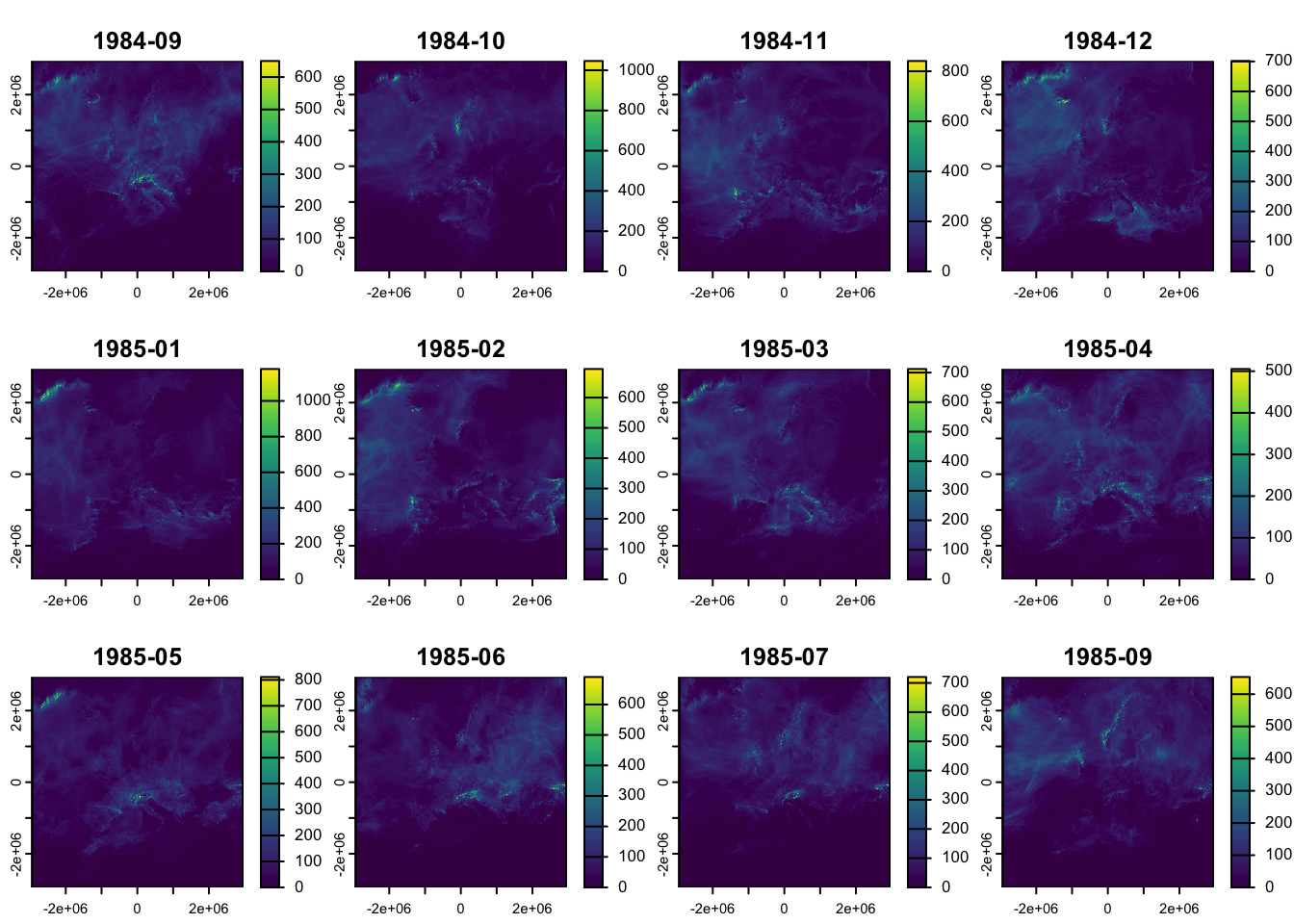

# visualize total precipitation on Sept 5th 1984 on a zoomable map 
plet(daily_sum[[5]])

b. Extract values for point locations

Here we extract the daily total precipitation for 12 centroids of Luxembourg provinces.

# extract daily accumulated rainfall for the centroids (point location) of each province in Luxembourg
v <- vect(system.file("ex/lux.shp", package = "terra"))  
v <- project(v,daily_sum) 
# convert polygons to points using their centroids
p <- terra::centroids(v)

# extract values from the above daily rasters 
values <- terra::extract(daily_sum,p,xy=TRUE)
# add province names 
values$province <- p$NAME_2

# Pivot longer: gather date columns into one
daily_rainfall <- values %>%
  pivot_longer(
    cols = -c(ID, x, y, province),
    names_to = "date",
    values_to = "value"
  ) %>%
  mutate(date = as.Date(date))

# daily rainfall per point 
ggplot(daily_rainfall, aes(x = date, y = value)) +
  geom_line(color = "darkgreen") +
  facet_wrap(~ province) +
  labs(title = "Daily Rainfall at Centroids of the provinces of Luxembourg",
       x = "Date", y = "Rainfall (mm)") +
  theme_minimal()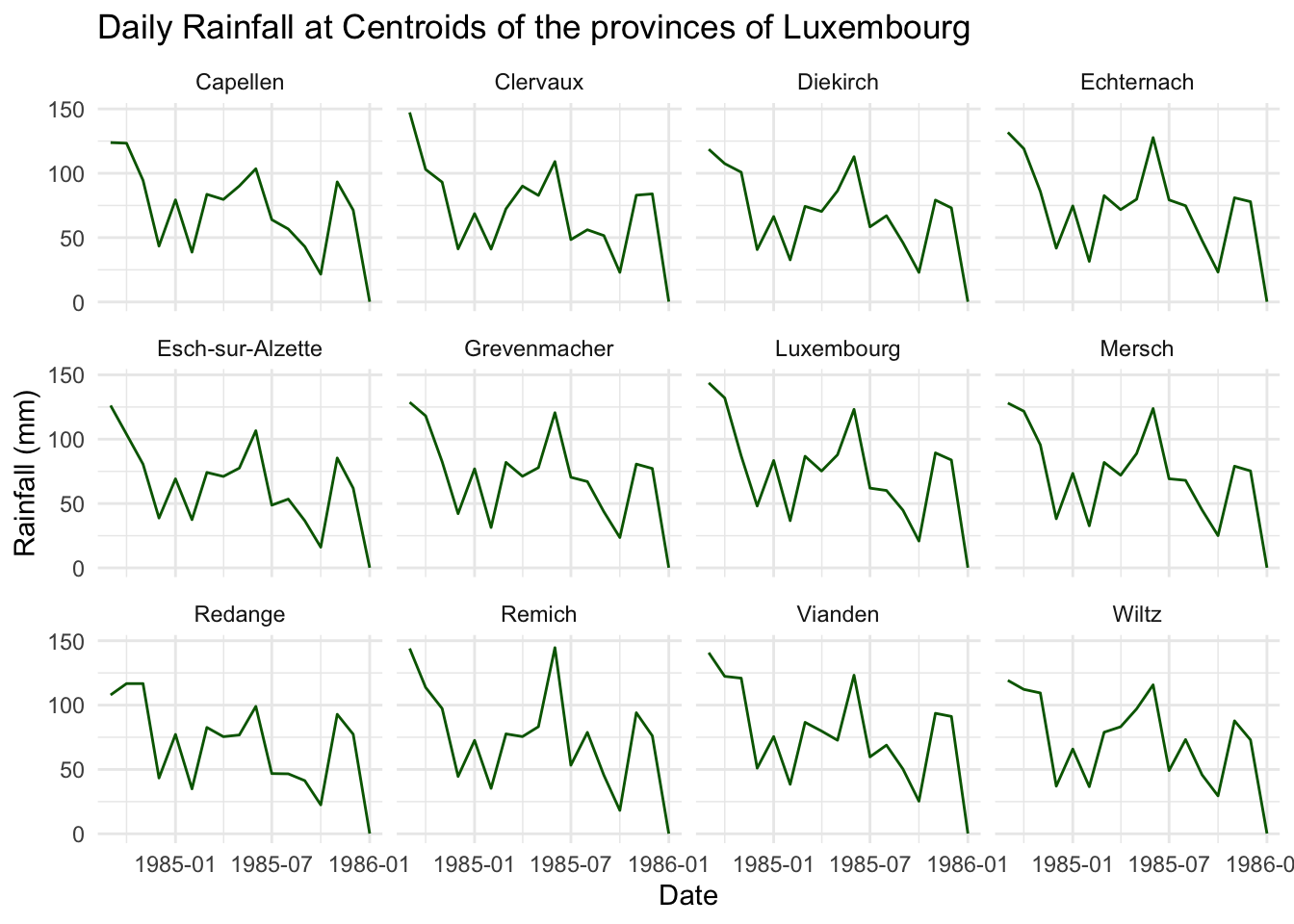

Conclusion

This script provides a complete automated workflow for downloading and processing total precipitation data from the CERRA dataset using CDS. It supports batch downloading, memory-optimized data handling, and time-based subsetting, making it suitable for long-term climatological analysis or integration into larger pipelines.

---