Data Management in RStudio

Introduction

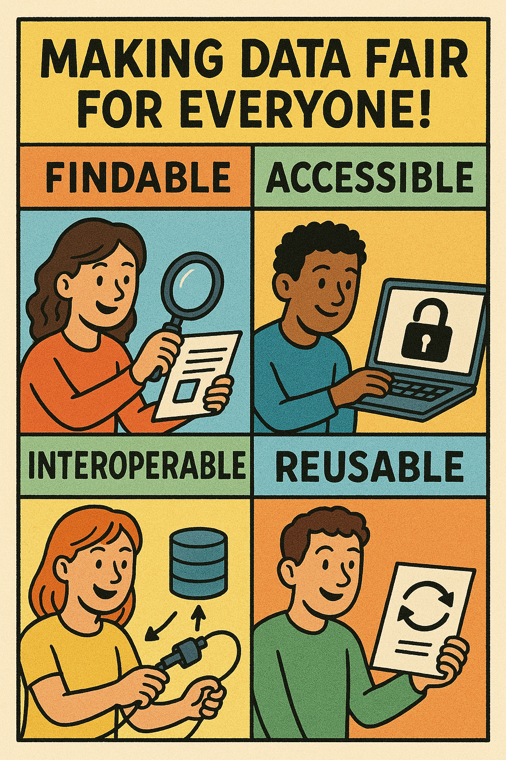
Reproducibility, transparency, and long-term usability of research outputs are increasingly crucial in science. To support these goals, the FAIR principles—Findable, Accessible, Interoperable and Reusable—provide a framework for organizing and sharing data and code. In this tutorial, we’ll learn how to manage a research project in RStudio in a way that aligns with FAIR principles.

Each section will include examples, exercises, and strategies to improve project, data and code organization. We’ll also explore how to set up Git and use it with RStudio for version control, as well as how to incorporate good metadata practices and open formats.

1. Directory structure and file naming

Start your project on the right foot! Organizing your files and directories effectively can save you countless hours and make collaboration so much more efficient. While there is no single “best” way to structure and name files, different methods may be more suitable for specific projects, depending on the nature of the work and personal preferences.

1.1 Directory structure

1.1.1 Informed, simple, structured and consistent

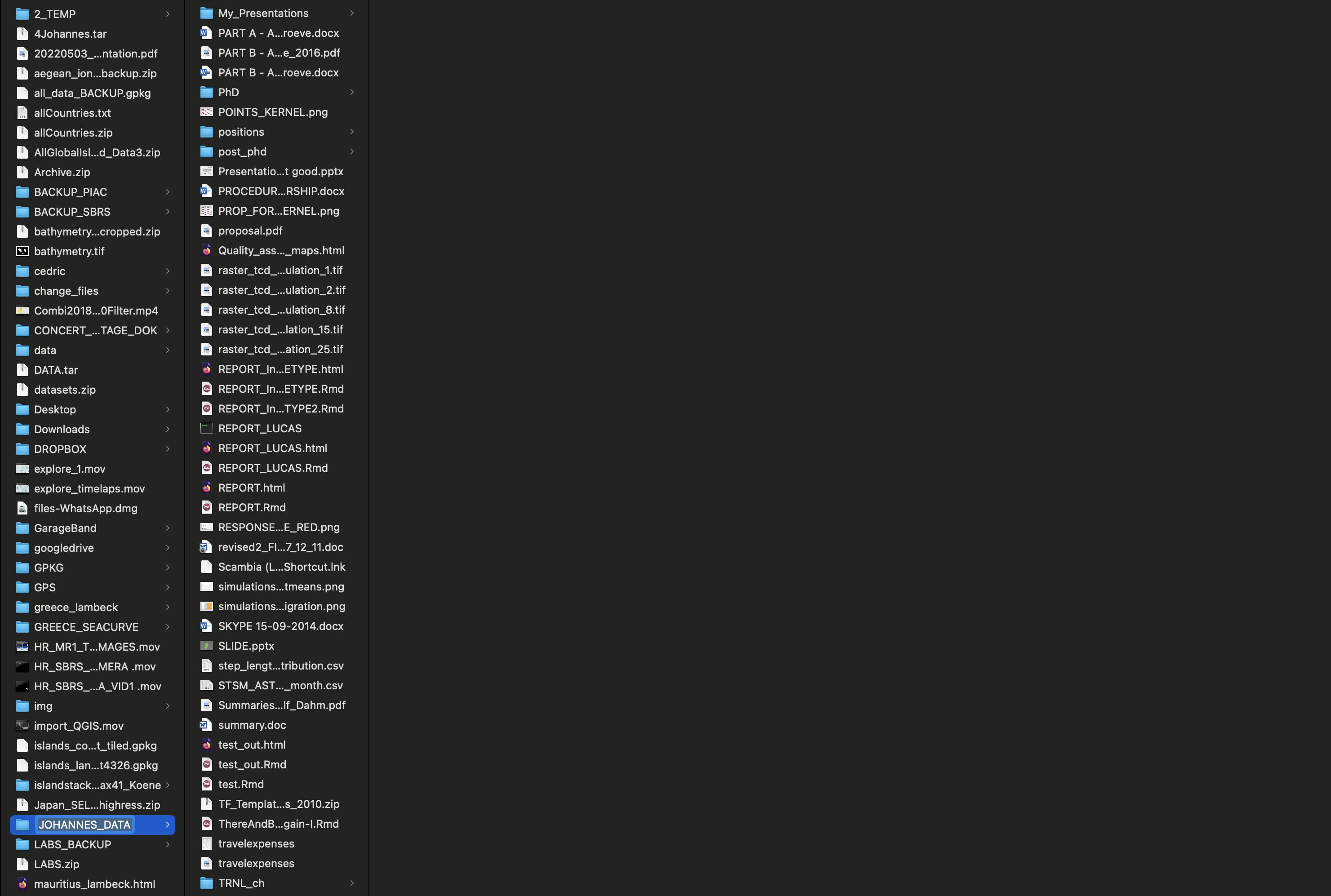
A common challenge faced by students and researchers is maintaining an organized project directory. The key to overcoming this is to start with a well-defined directory structure tailored to each individual project unit, such as a manuscript or thesis. This structure could be informed by your project proposal’s roadmap and Data Management Plan (DMP). While your project units and their requirements may evolve, having a clear starting point can provide a solid foundation for managing your data effectively.

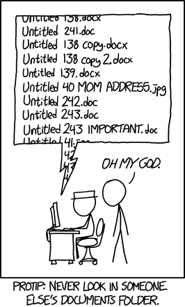
Let’s show you how not to do it.

Once upon a time…

Bad File Structure

This structure is disorganized, inconsistent, and difficult to maintain.

.
├── analysis final.R
├── final manuscript.docx
├── figs_final
│   ├── image1.png
│   └── image2.png
├── manuscript.docx
├── dataset.csv
├── output_results.xlsx
├── old/
│   └── backup_old_data_2021_final_FINAL.csv
├── notes.txt
├── temp/
│   ├── code_temp.R
│   └── temp2/
│       └── junk.R
└── working_dir/
    └── data analysis v2 (copy).R

Problems with the Bad Structure

Problem	Description
Files in root	Too many unrelated files make navigation hard.
Unclear naming	Files like `analysis final.R` and `dataset.csv` lack descriptive names.
Duplicate/confusing files	e.g., `final manuscript.docx` vs `manuscript.docx`.
Misuse of folders	Vague names like `temp`, `old`, `working_dir` lack purpose.
Manual versioning	`backup_old_data_2021_final_FINAL.csv` shows poor version control.
Special characters	Filenames like `data analysis v2 (copy).R` are difficult to reference.
No modular separation	Code, data, and outputs are not logically separated.

Good File Structure

This structure separates code, data, documents, and results clearly. It is easy to navigate, maintain, and share.

<project_name>
├── README.md
├── code/
│   ├── 00_<PROJ>_data-preparation.Rmd
│   └── 01_<PROJ>_analysis.Rmd
├── data/
│   ├── input/
│   └── output/
├── docs/
│   └── <PROJ>_manuscript.docx
├── figs/
└── project_name.Rproj

🇷 Are you curious how to print the above directory trees. You can use the R package fs.

install.packages('fs')
fs::dir_tree(path = ".", recurse = TRUE)

Exercise 1.1

Create a new project-directory on your PC and name it campaign2025 including a code, data, docs and figs directory.
Create an input and output directory as subdirectories in the data directory.
Print the directory tree using fs::dir_tree function in Rstudio.
TIP: specify the full name of the file path instead of path = "."

🇷 Are you curious how to generate the above directory structure in R?

# Approach 1 (create directories one-by-one) 

# Root directory 
if(!dir.exists('~/campaign2025')) 
  dir.create('~/campaign2025')

# Data directory 
if(!dir.exists('~/campaign2025/data')) 
  dir.create('~/campaign2025/data')
# create input and output directories in data
if(!dir.exists('~/campaign2025/data/input')) 
  dir.create('~/campaign2025/data/input')
if(!dir.exists('~/campaign2025/data/output'))
  dir.create('~/campaign2025/data/output')

# Create code, docs and figs directories
if(!dir.exists('~/campaign2025/code')) 
  dir.create('~/campaign2025/code')
if(!dir.exists('~/campaign2025/docs')) 
  dir.create('~/campaign2025/docs')
if(!dir.exists('~/campaign2025/figs')) 
  dir.create('~/campaign2025/figs')

# Generate directory tree
fs::dir_tree('~/campaign2025',recurse=TRUE)

# Approach 2 (use recursive to create all subdirectories simultaneously) 
if(!dir.exists('~/campaign2025/data/input')) 
  dir.create('~/campaign2025/data/input', 
             recursive = TRUE)
if(!dir.exists('~/campaign2025/data/output'))
  dir.create('~/campaign2025/data/output', 
             recursive = TRUE)

# Create code, docs and figs directories
if(!dir.exists('~/campaign2025/code')) 
  dir.create('~/campaign2025/code')
if(!dir.exists('~/campaign2025/docs')) 
  dir.create('~/campaign2025/docs')
if(!dir.exists('~/campaign2025/figs')) 
  dir.create('~/campaign2025/figs')
# Generate directory tree
fs::dir_tree('~/campaign2025',recurse=TRUE)

1.1.1 Case study: Camera trapping images

1.1.1.1 Main data directory

Suppose we have camera trapping images coming from two camera traps for a campaign in 2025 and the aim is to identify the species in those images.
(1) In which directory could we place the raw images and (2) where could we store identified species from the images? How would you name the directories and subdirectories?

.
├── README.md
├── code/
├── data/
├── docs/
├── figs/
└── project_name.Rproj

Option 1

Here we decide to store images in a directory named img in input and species_observations in the output.

.
├── README.md
├── code/
├── data/
│   ├── input/
│   │   └── img/
│   └── output/
│       └── species_observations/
├── docs/
├── figs/
└── project_name.Rproj

Option 2

Here we decide to store images in a directory named img in raw and species_observations in the processed.

.
├── README.md
├── code/
├── data/
│   ├── raw/
│   │   └── img/
│   └── processed/
│       └── species_observations/
├── docs/
├── figs/
└── project_name.Rproj

1.1.1.2 Subdirectories

Further partitioning of a dataset might be relevant. For instance, camera traps might result in thousands of images. Dumping everything into one folder makes navigation slow and error-prone. It makes it harder to sort or retrieve specific files without scanning all file names or metadata, which will become an issue when there are a lot of files. By organizing files by metadata (e.g., camera ID, date), it becomes much easier to search, filter, or batch process. It also facilitates archiving, for instance, making a monthly zipped backup. For making a further partitioning of your data into directories, think about relevant metadata (e.g., date, technique, collector, site, parameter settings) that could be used to partition the data.

How could you further partition the camera trap images, currently stored in data/input/img/DEVICEID/?

Images organized by camera → Date (YYYYMMDD)

data/input/img/DEVICEID/YYYYMMDD/

./data/input/
└── img/
    ├── cam001/
    │   ├── 20250801/
    │   └── 20250802/
    └── cam002/
        ├── 20250801/
        └── 20250803/

Images organized by camera → Date (YYYY/MM/DD)

data/input/img/DEVICEID/YYYY/MM/DD/

./data/input/
└── img/
    ├── cam001/
    │   └── 2025/
    │       └── 08/
    │           ├── 01/
    │           └── 02/
    └── cam002/
        └── 2025/
            └── 08/
                ├── 01/
                └── 03/

Deployment

An important addition to the camera trap image directory structure is the location or site of each camera. Since cameras may be moved over time, it’s useful to define a deployment as the combination of site, device, and monitoring period (start and end time). This concept helps track where and when a specific device was recording and is central to organizing data from any type of monitoring equipment. If devices are expected to move between locations, it can be useful to structure the directory around deployments—grouping images by both site and device ID.

For devices without a fixed location, such as GPS and accelerometer collars, a deployment typically refers to the combination of individual, device, and monitoring period.

Images Organized by site and device ID (YYYY/MM/DD)

data/input/img/SITEID/DEVICEID/YYYY/MM/DD/

./data/input/
└── img/
    ├── site001/
    │   └── cam001/
    │       └── 2025/
    │           └── 08/
    │               ├── 01/
    │               └── 02/
    └── site002/
        └── cam002/
        │   └── 2025/
        │       └── 08/
        │           ├── 01/
        │           └── 03/
        └── cam001/
            └── 2025/
                └── 09/
                    ├── 01/
                    └── 03/

Images Organized by device and site ID (YYYY/MM/DD)

data/input/img/DEVICEID/SITEID/YYYY/MM/DD/

./data/input/
└── img/
    ├── cam001/
    │   └── site001/
    │   │   └── 2025/
    │   │       └── 08/
    │   │           ├── 01/
    │   │           └── 02/
    │   └── site002/
    │       └── 2025/
    │           └── 09/
    │               ├── 01/
    │               └── 03/
    └── cam002/
        └── site002/
            └── 2025/
                └── 08/
                    ├── 01/
                    └── 03/

1.1.2 R Projects

R Projects are a foundational tool for good project management in RStudio. They isolate your work into a self-contained environment, avoiding messy workspaces. R provides many options to keep your project organized and at the foundation is the R project (.Rproj) file.

Exercise 1.2

Open RStudio and create a new R Project (File > New Project).
1. Choose existing directory and navigate to campaign2025.
2. Close RStudio, navigate to campaign2025 and open the R project by clicking the .Rproj file.
3. Check the current working directory with getwd().
  Cool, the current working directory is the root of the project!
4. Is there another way how to open your R project?
5. Create the img directory in the input directory.
6. Create the subdirectory structure using the following directory structure: ./data/input/img/DEVICEID/YYYYMMDD/
  
  For device id cam001: 2025-08-01, 2025-08-03
  For device id cam002: 2025-08-01
```
./data/input/
└── img/
    ├── cam001/
    │   └── 2025/
    │       └── 08/
    │           ├── 01/
    │           └── 02/
    └── cam002/
        └── 2025/
            └── 08/
                ├── 01/
                └── 03/
```
7. Print the directory tree using fs::dir_tree().
  TIP: Since you are working within an .rproj there is no need to specify the file path as we did in exercise 1.1.
Explore other R project options (File > New Project > New Repository > … )

🇷 Are you curious how to auto-generate the above directory structure?

Here an example is given on how to create a directory structure organized by device ID and YYYY/MM/DD: data/input/img/DEVICEID/YYYY/MM/DD/

# main directory for images 
img_dir <- './data/input/img'
  
# generate dates of the year 
dates <- seq(as.Date('2025-01-01'), 
             as.Date('2025-12-31'),
             '1 day')
head(dates,5)
# device identifiers 
(device_ids <- c('cam001','cam002'))

# convert YYYY-MM-DD to YYYYMMDD for directory partitioning 
dates_dir <- gsub('-','/',dates) # substitute '-' by '/'
head(dates_dir,5)

# generate directories 
for(j in 1:length(device_ids)){ 
  message(device_ids[j])
  for(i in 1:length(dates_dir)){
    # create directories for dates for every device id
    dirs <- paste(img_dir,
                  device_ids[j],
                  dates_dir[i],
                  sep='/')
    message(dirs)
    if(!dir.exists(dirs)){
    dir.create(dirs,recursive=TRUE)
    }
  }
}
 
# example of the last directory created by the loop
print(dirs)

# explore the directory tree 
fs::dir_tree(path = img_dir, recurse = 2) # months

Exercise 1.3

Copy-paste the above code and paste it in a new R script in your project.
Save the script in the code directory and name it 00_create_dir_tree.R.
Run the code line-by-line, read the comments and explore the output in the console after running each line.
Explore the ./data/input/img/ directory and see how year, month and day directories have been magically created.
Go back to the script 00_create_dir_tree.R and identify what needs to be changed in the code if you would want to generate the directory structure YYYYMMDD instead of YYYY/MM/DD?
TIP: read the comments attentively! One character only needs to be changed.

a. After making the change, print the first 10 date directories (dates_dir) using the head() function to see if the directories will indeed be defined correctly as YYYYMMDD.

b. Re-run the for-loop (for (j in ...){}) after changing the script.

c. Explore the ./data/input/img/ directory and see how date directories have been magically created.

d. Remove the YYYYMMDD directories.

1.2 File naming

1.2.1 Metadata is key

Organizing files using clear, consistent, and meaningful names is essential for ensuring long-term accessibility, reproducibility, and collaboration. A well-designed naming convention makes it easier to locate, understand, and process files—both for humans and machines. File naming may go hand-in-hand with the directory structure. For file naming, you could think about the relevant metadata (e.g., date, technique, collector, parameter settings) that should be included to non ambiguously identify files. Make sure that files which belong to a single data type or dataset are consistently named, using the same naming patterns (order of metadata information in the filename). Following such practices not only support good data management but also interoperability across systems and platforms. By naming and structuring your files consistently, your dataset becomes machine-readible and computational analysis is facilitated.

1.2.2 Case study: Camera trapping images

Here is an example of the file naming for the camera case study presented above.

Image names including device ID and timestamp (YYYYMMDDhhmmss)

data/input/img/DEVICEID/YYYYMMDD/DEVICEID_YYYYMMDDhhmmss.png

./data/input/
└── img/
    ├── cam001/
    │   ├── 20250801/
    │   │   ├── cam001_20250801123000.png
    │   │   └── cam001_20250801124500.png
    │   └── 20250802/
    │       └── cam001_20250802103000.png
    └── cam002/
        ├── 20250801/
        │   └── cam002_20250801131500.png
        └── 20250803/
            └── cam002_20250803120000.png

Image names including device and site ID and timestamp (YYYYMMDDhhmmss)

data/input/img/DEVICEID/YYYYMMDD/DEVICEID_SITEID_YYYYMMDDhhmmss.png

./data/input/
└── img/
    ├── site001/
    │   └── cam001/
    │       └── 2025/
    │           └── 08/
    │               ├── 01/
    |               │   ├── cam001_site001_20250801123000.png
    │               │   └── cam001_site001_20250801124500.png
    │               └── 02/
    │                   └── cam001_site001_20250802103000.png
    └── site002/
        └── cam002/
            └── 2025/
                └── 08/
                    ├── 01/
                    │   └── cam002_site002_20250801131500.png
                    └── 03/
                        └── cam002_site002_20250803120000.png

🇷 Listing your datasets in R can be done with the function list.files()

All file names follow a consistent naming convention, which is very useful for parsing and automation. Dates are formatted using the standard YYYYMMDD pattern, and timestamps as YYYYMMDDhhmmss. Device identifiers use the prefix cam followed by a zero-padded number. This convention ensures all file names are of equal length, making them easier to sort and process programmatically.

# list all images 
list.files(path = "./data/input/img", 
           recursive = TRUE, 
           full.names = TRUE)
[1] "data/input/img/cam001/20250801/cam001_20250801123000.png"
[2] "data/input/img/cam001/20250801/cam001_20250801124500.png"
[3] "data/input/img/cam001/20250802/cam001_20250802103000.png"
[4] "data/input/img/cam002/20250801/cam001_20250801131500.png"
[5] "data/input/img/cam002/20250803/cam001_20250803120000.png"

# list images from one specific date
list.files(path = "./data/input/img", 
           pattern= '20250801'
           recursive = TRUE, 
           full.names = TRUE)
[1] "data/input/img/cam001/20250801/cam001_20250801123000.png"
[2] "data/input/img/cam001/20250801/cam001_20250801124500.png"
[4] "data/input/img/cam002/20250801/cam001_20250801131500.png"

# list images from one specific device
list.files(path = "./data/input/img/cam001", 
           pattern= '20250801'
           recursive = TRUE, 
           full.names = TRUE)
[1] "data/input/img/cam001/20250801/cam001_20250801123000.png"
[2] "data/input/img/cam001/20250801/cam001_20250801124500.png"
[3] "data/input/img/cam001/20250802/cam001_20250802103000.png"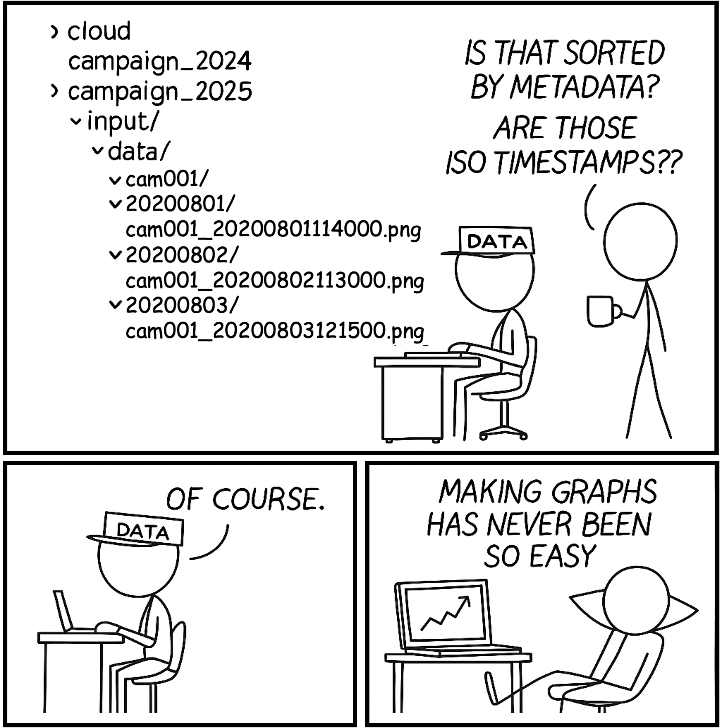

1.2.3 General file naming rules

Naming is not only relevant for data but also for scripts and outputs (figures, tables). Make sure that those also have intuitive and meaningful names. Here we list some general good practices for determining file names.

1.2.3.1 Computer-readable file names

What makes a file name computer-readable? First, computer readable files contain no spaces, no punctuation, and no special characters. They are case-consistent, which means that you always stick to the same case pattern, whether that be full lowercase, camel case (ThisIsWhatIMeanByCamelCase), or whatever else. Finally, good file names make deliberate use of text delimiters. Wise use of delimiters makes it easy to look for patterns when you are searching for a specific file. Usually, it’s recommended that you use an underscore (_) to delimit metadata units and a dash (-) to delimit words within a metadata unit. For example, here is a good, computer-readable file name:

ori_day01_data-management.qmd

1.2.2.2 Human-readable file names

The example file name above is not only computer-readable, it’s also human-readable. This means that a human can read the file name and have a pretty good idea of what’s in that file. Good file names are informative! You shouldn’t be afraid to use long names if that’s what it takes to make them descriptive.

1.2.2.3 File names that work well with default ordering

If you sort your files alphabetically in a folder, you want them to be ordered in a way that makes sense. Whether you sort your files by date or by a sequential number, the number always goes first. For dates, use the YMD format, or your files created in April of 1984 and 2020 will be closer than the ones created in March and April 2020. If you are using sequential numbering, add a sensible amount of zeros in front based on how many files of that category you expect to have in the future. If you expect to have more than 10 but not more than 99 files, you can add a single leading zero (e.g., “data_analysis_01.R” instead of “data_analysis_1.R”), whereas if you expect to have between 100 and 999 you can add two (e.g., “Photo_001.jpeg” instead of “Photo_1.jpeg” or “Photo_01.jpeg”).

.
├── README.md
├── code/
│   ├── 00_campaign2025_image-preparation.Rmd
│   └── 01_campaign2025_species-observations.Rmd
├── data/
│   ├── input/
│   │   ├── cam001/
│   │   │   ├── 20250801/
│   │   │   │   ├── cam001_20250801123000.png
│   │   │   │   └── cam001_20250801124500.png
│   │   │   └── 20250802/
│   │   │       └── cam001_20250802103000.png
│   │   └── cam002/
│   │       ├── 20250801/
│   │       │   └── cam002_20250801131500.png
│   │       └── 20250803/
│   │           └── cam002_20250803120000.png
│   └── output/
│       └── 01_species-observations/
|           └── 01_species-observations.csv 
├── docs/
├── figs/
└── campaign2025.Rproj

Exercise 1.4

Search for 5 images on the web and save them in the respective directories including the device id (cam001, cam002) and date time (YYYYMMDDhhmmss) as the filename. Use an underscore (_) to separate different metadata fields in the filename. Store them in their corresponding directories.

Resting male lion (cam001, 2025-08-01 12:30:00)
Browsing Giraffe (cam001, 2025-08-01 12:45:00),
Running African Wild dog (cam001, 2025-08-02 10:30:00)
Hunting female lion (cam002, 2025-08-01 13:15:00)
Digging African Elephant (cam002, 2025-08-03 12:00:00)
Use list.files('./data/input/img',recursive=TRUE, full.names=TRUE) to list all the image names. Do you see any inconsistencies? In case you find mistakes, correct it!
Use list.files() to only list image names from 2025-08-01. See examples of the usage of list.files above.

1.3. Tips for Good File and Directory Organization

Here, we provide practical guidelines to help you establish a consistent and efficient approach to naming files and directories. These examples are designed to be simple yet adaptable to suit your project’s specific needs.

Key Guideline	Short Description	Long Description
Organize by Relevant Metadata	Sort files by compound, technique, date, or collector.	Sort files in directories based on essential metadata such as compound, technique, date, or person collecting the data. This enhances findability and maintains consistency across your dataset.
Establish Clear Naming Conventions	Create a well-defined naming system for directories and files.	Define a consistent and intuitive naming convention. Ensure collaborators or users understand and follow the structure to maintain data integrity and usability.
Fully Describe File Contents in Filenames	Include key details in filenames for easy identification.	Filenames should clearly describe file contents. Avoid cryptic or overly abbreviated names and include relevant metadata (e.g., date, device ID, location).
Use ISO 8601 Date Format	Adopt the YYYYMMDD date format for filenames.	Always use the ISO 8601 format (e.g., `20250801`) to make sorting and searching easier. This format supports consistent chronological order in file listings.
Avoid Special Characters and Spaces	Use underscores instead of spaces or special characters.	Avoid using characters like `@`, `#`, `&`, or spaces. Use `_` or `-` instead. This improves compatibility across systems and ensures scripts or programs can access files without issues.
Separate Raw and Processed Data	Distinguish between original and derived data.	Maintain clear directory separation between raw (unmodified) and processed (cleaned or transformed) data. This improves reproducibility and protects original data.
Avoid Duplicate and Vague Filenames	Do not use names like `final_v2_REAL.docx`.	Choose specific, descriptive filenames instead of vague or redundant ones. Manual versioning leads to confusion and lost data. Use automated version control when possible.
Use Version Control	Use Git or similar tools instead of manual backups.	Replace file duplication with proper version control. Git provides reliable history, collaboration support, and change tracking without cluttering directories.

2. Spreadsheets

2.1 What are spreadsheets good for?

Spreadsheets are good tools for data entry. Even though you could technically run some data analyses within your spreadsheet program, that doesn’t mean you should! The main downside to doing data processing and analysis in a spreadsheet is that it entails a lot of pointing and clicking. This makes your analysis difficult to reproduce. If you need to re-run your analysis or re-process some data, you have to do it manually all over again. Also, if you go back to your completed analysis after a while (for example to write the methods of your paper) and you don’t remember what you did, there is no record of it left. This is why spreadsheets are introduced exclusively as a tool for data entry.

2.2 Human-readable vs. computer-readable data

Most of the problematic practices outlined in this Chapter can be summarized into a single concept: using spreadsheets to convey information in a way that is readable for humans but not for computers. While a human brain is capable of extracting information from context, such as spatial layout, colors, footnotes, etc., a computer is very literal and does not understand any of that. To make good use of spreadsheets, we need to put ourselves in the computer’s mind. All the computer understands from a spreadsheet is the information encoded in rows and columns. So, the number one rule to remember when using spreadsheets is to make your data “tidy”.

2.3 Tidy data

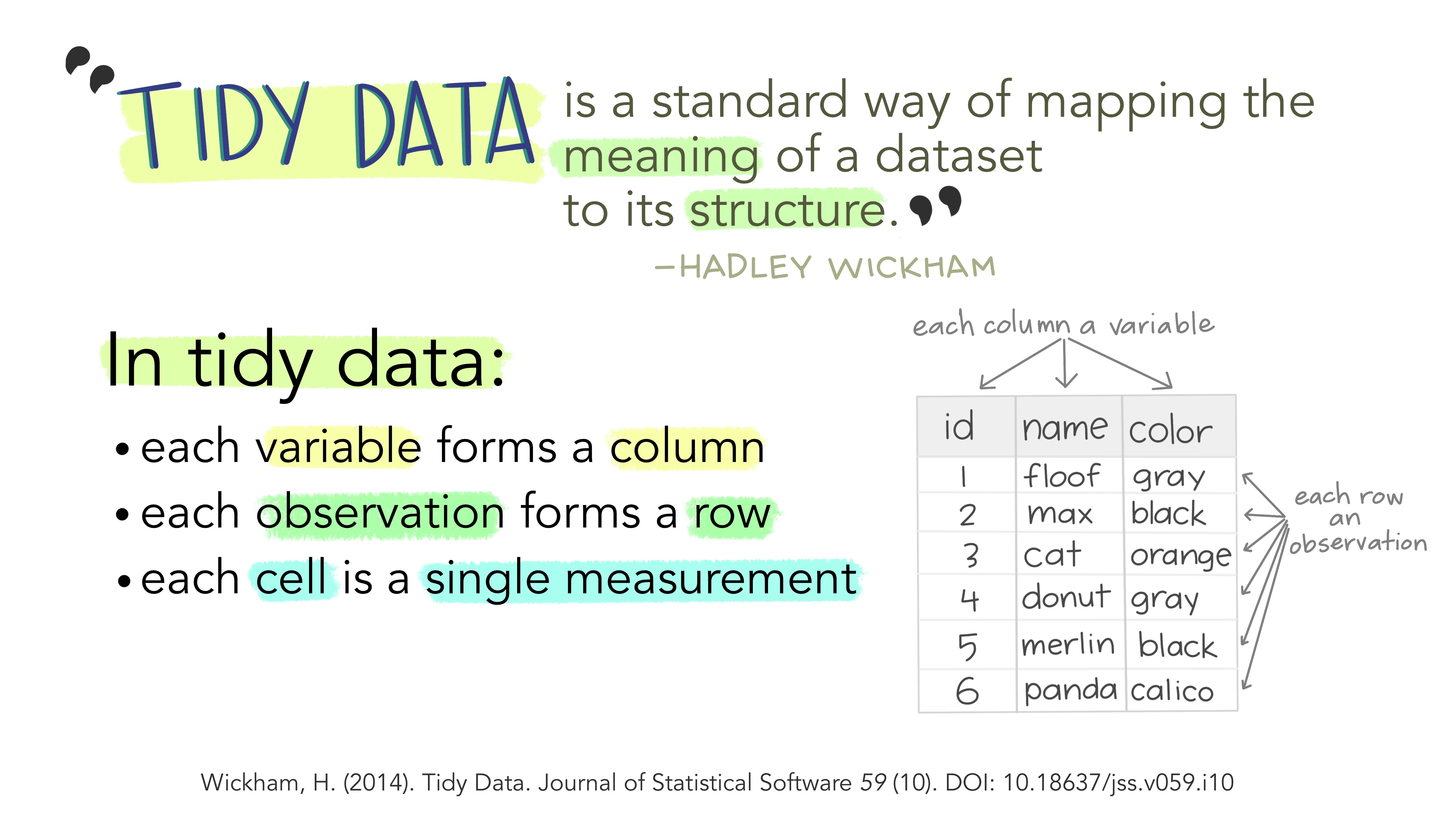
The fundamental definition of tidy data is quite simple: one variable per column and one observation per row. Variables are the things we are measuring (e.g., temperature, distance, height). Observations are repeated measurements of a variable on different experimental units. Structuring your data following this rule will put you in a great position for processing and analyzing your data in an automated way. First, using a standard approach to formatting data, where the structure of a table reflects the meaning of its content (i.e., where a column always means a variable and a row always means an observation) removes any ambiguity for yourself and for the computer. Second, this specific approach works very well with programming languages, like R, that support vector calculations (i.e., calculations on entire columns or tables at a time, instead of single elements only).

2.4 Problematic practices

In practice, what are some common habits that contradict the principles of tidy data? Here are some examples.

2.4.1 Multiple variables in a single column

Putting information for two separate variables into one column contradicts the “one column per variable” principle. A classic example of this is merging age class and sex into one – for example “adult female”, “juvenile male”, etc. If, for instance, later on we wanted to filter based on age only, we would have to first separate the information within the column and then apply a filter. It is much more straightforward to combine information than to split it, so the structure of our data should always follow a reductionist approach where each table unit (cell) contains a single data unit (value).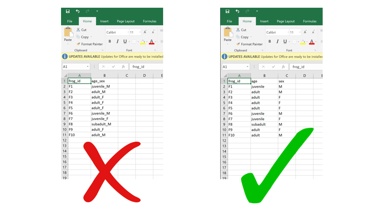

2.4.2 Rows for variables, columns for observation

While the choice of using rows for observations and columns for variables may seem arbitrary – after all, why can’t it be the other way around? – consider this: the most commonly used data structure in R, the data frame, is a collection of vectors stored as columns. A property of vectors is that they contain data of a single type (for instance, you can’t have both numbers and characters in the same vector, they either have to be all numbers or all characters). Now imagine a situation where a dataset includes weight measurements of individual green frogs captured in different ponds: for each frog, we’d have a weight value (a number) and the name of the pond where it was captured (a character string). If each frog gets a row, we get a column for weight (all numbers) and a column for pond (all characters). If each frog gets a column and weight and pond go in different rows, each column would contain a number and a character, which is not compatible with R. This is valid not only for R, but for other vector-based programming languages too. The tidy data format makes sure your data integrates well with your analysis software which means less work for you getting the data cleaned and ready.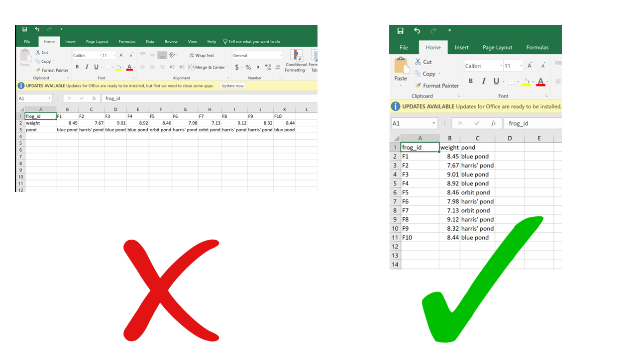

2.4.3 Multiple tables in a single spreadsheet

Creating multiple tables in a single spreadsheet is problematic because, while a human can see the layout (empty cells to visually separate different tables, borders, etc.) and interpret the tables as separate, the computer doesn’t have eyes and won’t understand that these are separate. Two values on the same row will be interpreted as belonging to the same experimental unit. Having multiple tables within a single spreadsheet draws false associations between values in the data. Starting from this format will invariably require some manual steps to get the data into a format the computer will read. Not good for reproducibility!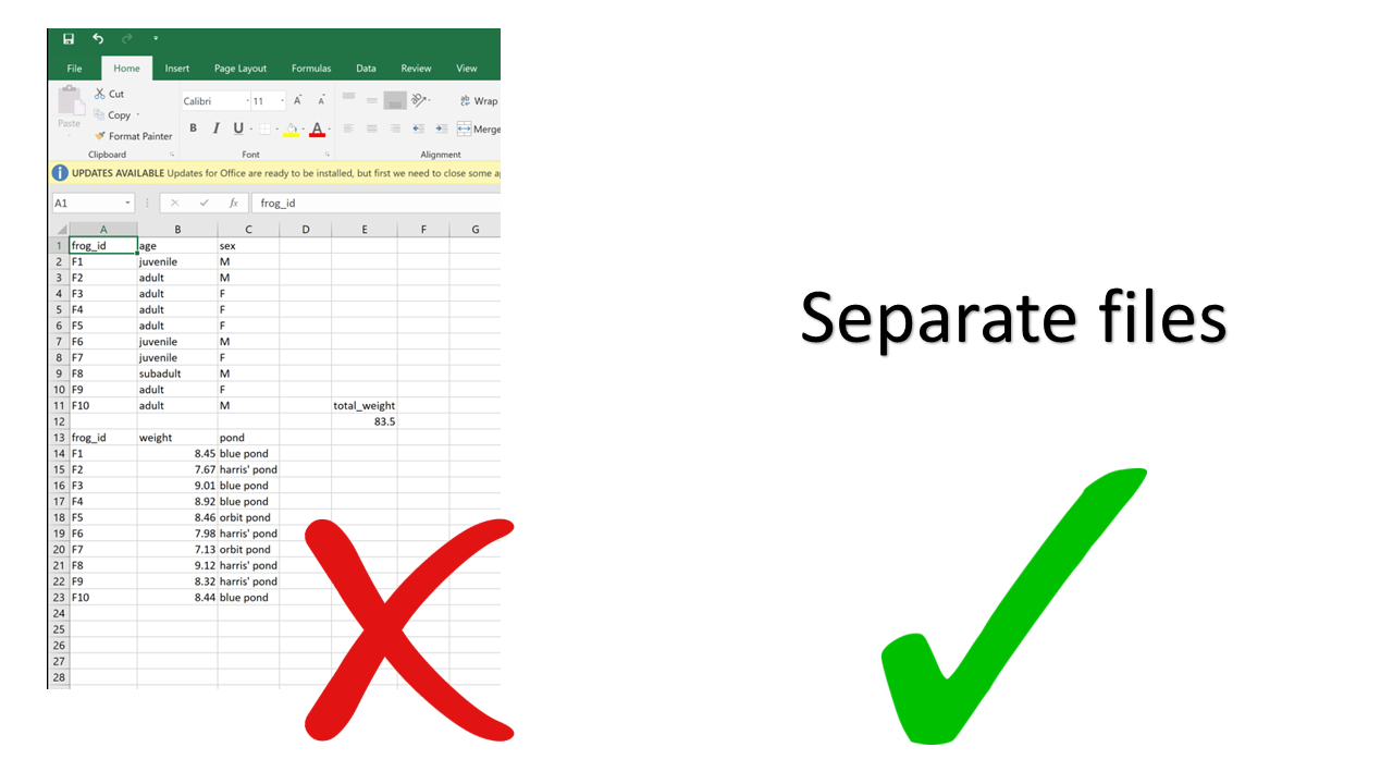

2.4.4 Multiple sheets

This one may seem innocuous, but actually it can be problematic as well. For starters, you can’t load multiple sheets into R at the same time (by multiple sheets, I mean the tabs at the bottom). If you’re only using base R functions, you can’t even load a .xslx file (although you can using packages such as readxl), so you’re going to have to save your spreadsheets as .csv before importing. When saving as .csv, you’ll only be able to save one sheet at a time. If you’re not aware of this, you end up losing track of the data that was in the other sheets. Even if you are aware, it just makes it more work for you to save each of the sheets separately.

Using multiple sheets becomes even more of a problem when you are saving the same type of information into separate sheets, like for example the same type of data collected during different surveys or years. This contradicts another principle of tidy data, which is each type of observational unit forms a table. There’s no reason to split a table into multiple ones if they all contain the same type of observational unit (e.g., morphometric measurements of frogs from different ponds). Instead, you can just add an extra column for the survey number or year. This way you avoid inadvertently introducing inconsistencies in format when entering data, and you save yourself the work of having to merge multiple sheets into one when you start processing and analyzing.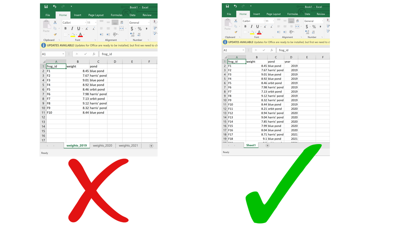

2.4.5 Using formatting to convey information

Anything that has to do with visual formatting is not computer-readable. This includes borders, merging cells, colors, etc. When you load the data into an analysis software, all the graphical features are lost and all that is left is… rows and columns. Resisting the temptation to merge cells, and instead repeating the value across all rows/columns that it applies to, is making your data computer-friendly. Resisting the urge to color-code your data, and instead adding an additional column to encode the information you want to convey with the different colors, is making your data computer-friendly. Columns are cheap and there’s no such thing as too many of them.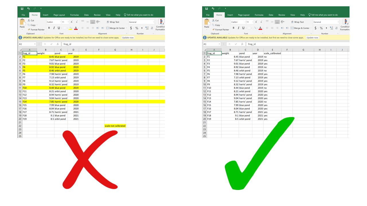

2.4.6 Putting units in cells

Ideally, each measurement of a variable should be recorded in the same units. In this case, you can add the unit to the column name. But even if a column includes measurements in different units, these units should never go after the values in the cells. Adding units will make your processing/analysis software read that column as a character rather than as a numeric variable. Instead, if you need to specify which unit each measurement was taken in, add a new column called “variable_unit” and report it there. Remember, columns are cheap!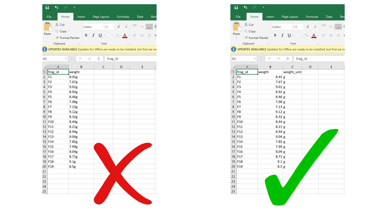

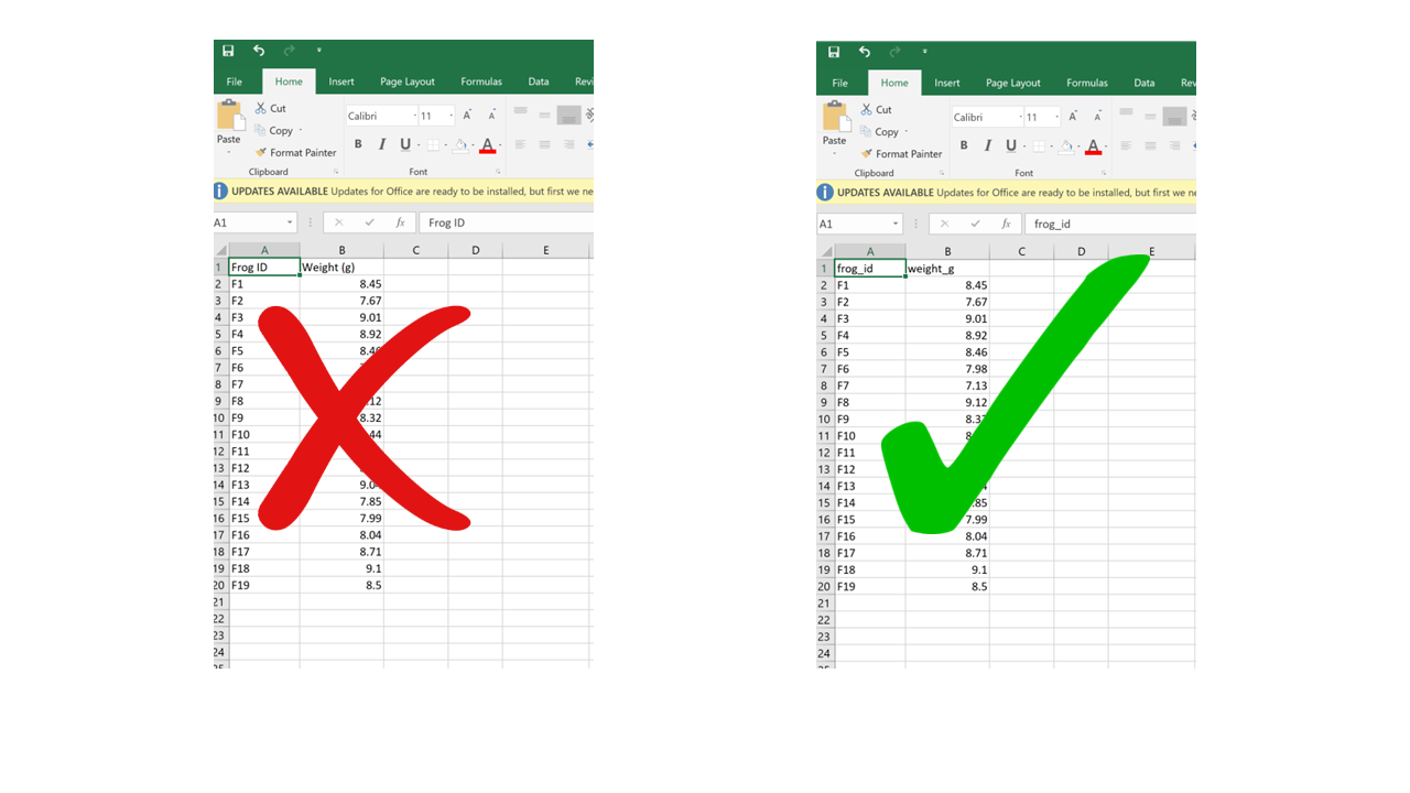
2.4.7 Using problematic column names

Problematic column names are a lot like the problematic file names from Chapter 1. They are non-descriptive, they contain spaces or special characters – in short, they are human-readable but not computer-readable. Whether you separate words in column names using camel case or underscores, avoid using spaces. It’s a good idea to include units in the column names, e.g., “weight_g”, “distance_km”, etc. Also, just like for file names, be consistent in your capitalization pattern and choice of delimiters.

2.4.8 Conflating zeros and missing values

Conflating zero measurements with missing values by using a zero or a blank cell as interchangeable is a problem, because there’s a big difference between something you didn’t measure and something that you did measure and it was zero. Any blank cell will be interpreted as missing data by your processing/analysis software, so if something is zero it needs to be actually entered as a zero, not just left blank. Similarly, never use zero as your value for missing data. These are two separate meanings that need to be encoded with different values.

2.4.9 Using problematic null values

Many common ways to encode missing values are problematic because processing/analysis software does not interpret them correctly. For example, “999” or “-999” is a common choice to signify missing values. However, computers are very literal, and those are numbers. You may end up accidentally including those numbers in your calculations without realizing because your software did not recognize them as missing values. Similarly, like we said, “0” is indistinguishable from a true zero and should never be used to signify “missing data”. Worded options, such as “Unknown”, “Missing”, or “No data” should be avoided because including a character value into a column that is otherwise numeric will cause the entire column to be read as character by R, and you won’t be able to do math on the numbers. Using the native missing value encoding from your most used programming language (e.g., NA for R, NULL for SQL, etc.) is a good option, although it can also be interpreted as text in some instances. The recommended way to go is to simply leave missing values blank. The downside to this is that, while you’re entering data, it can be tricky to remember which cells you left blank because the data is missing and which ones are blank because you haven’t filled them yet. Also, if you accidentally enter a space in an empty cell, it will look like it’s blank when it actually is not.

2.4.9.1 Inconsistent value formatting

A very common problem arises when having to filter/tally/organize data based on a criterion that was recorded inconsistently in the data. I find this to be especially common for columns containing character-type variables. For example, if the person entering data used “F” or “Female” or “f” interchangeably in the “sex” column, it will be difficult later on to know how many female individuals are in the dataset. Similarly, if the column “observer” contains the name of the same person written in multiple different ways (e.g., “Mary Brown”, “Mary Jean Brown”, “M. Brown”, “MJ Brown”), these won’t be recognized as the same person unless these inconsistencies are fixed later on.

2.5 Document

If you follow all the guidelines outlined in this Chapter, chances are you will be able to automate all of your data processing without having to do anything manually, because the data will be in a computer-readable format to begin with. However, if you do end up having to do some manual processing, make sure you thoroughly document every step: Never edit your raw data; save processed/cleaned versions as new files; and describe all the steps you took to get from the raw data to the clean data in your README file.

Exercise 2.1

Find the mistakes in 01_species_observations_bad .xlsx.
Standardize variable names, data types, and date formats.
Copy the file 01_species_observations.csv into your own project into a directory: data/output/01_species_observations
Where would you save a derived count table of the number of species and how would you name the table?

solution

Merged fields: Device+Site, SexAge, Species (Latin/English)
Inconsistent species formatting: mix of languages and casing (Vulpes vulpes / Red fox, Vulpes Vulpes / RED FOX)
Units inside cells: coordinates include EPSG (4.123, 52.123 (EPSG:4326))
Mixing of data types: ?
wrong notation of missing values: ?/MISSING instead of NA
Formatting-as-data: bold text, color highlighting
Non-standard date/time: 01-08-25 12:30 (ambiguous order, not ISO)
Several tables in same sheet: observations above, species/diet counts below separated by empty rows

# output directory 
output_dir <- './data/output/01_species_observations/'

# import species observations 
species_observations <- read.table(paste0(output_dir,'01_species_observations.csv'),
                                   sep=';',
                                   header=TRUE)

# counts per species 
counts_per_species <- plyr::count(species_observations$species_name)

# create output directory 
if(!dir.exists(output_dir)){
  dir.create(output_dir)
}

# export table 
write.table(counts_per_species,
            paste0(output_dir,'01_counts_per_species.csv'),
            row.names = FALSE)

Exercise 2.2

Copy-paste the solution in a new script named 01_species_observations.R in the code directory and run it. It will create a csv in the directory data/output/01_species_observations/ named 01_counts_per_species.csv

3. Code Management

In research, writing clear and well-structured scripts is critical for ensuring reproducibility, transparency, and collaboration in scientific studies. Following coding best practices can save time, reduce errors, and make your analyses more accessible to others.

It is highly recommended to use code for all processing steps, from data preparation, data filtering & extraction to the final analysis. By writing scripts for these tasks, you ensure that the raw data remains untouched while creating a reproducible workflow. This approach avoids relying on proprietary software, which may offer convenience but often uses file formats and processing steps that are not easily replicated. By embracing coding, you align your workflows with open science principles, ensuring your data and results are accessible, transparent, and reusable - which can ultimately be used to validate your research.

Learning to code may feel like a steep curve at first, but the effort is highly rewarding. As you develop your skills, you’ll gain the ability to automate tasks, handle large datasets more efficiently, and collaborate with others more effectively. For those new to coding, starting with simple steps like organizing code by projects, adding comments and using clear names for variables and functions can significantly improve your scripts. As you become more comfortable, adopting tools like version control systems or writing modular code can further enhance your workflow and facilitate collaboration in larger projects. These best practices are designed to help you produce reliable, reusable, and efficient code for your research.

3.1. Comment your code

Good comments make code easier to understand, both for others and for your future self. A well-placed comment can explain the purpose of a block of code, clarify why a particular approach was chosen, or note important assumptions. Comments should not simply restate what the code already says — for example, writing # add 1 to x above x <- x + 1 adds no real value. Instead, focus on making your comments informative, explaining why you are doing something or summarizing the logic of a more complex section. Placing short, clear comments throughout your script can greatly reduce the time needed to understand or debug it later.

Example:

# Filter dataset to only include adult individuals (age >= 18)
# This is necessary because juveniles have incomplete measurements
adults <- data[data$age >= 18, ]

3.2. Use a style guide

A consistent coding style improves readability and makes it easier for multiple people to work on the same project. This means following common conventions for naming variables, structuring code, and formatting scripts. A style guide also helps you avoid small but frustrating inconsistencies, such as mixing spaces and tabs or switching between different naming conventions. Adopting a style guide early in a project ensures that everyone writes code in the same way, making collaboration smoother and reducing misunderstandings. For R, you can refer to the Hadley Wickham R Code Style Guide, which provides practical examples and recommendations.

3.3. Functions

Functions are one of the most effective ways to make code reusable, readable, and easy to maintain. They are particularly valuable for tasks that you need to repeat or that logically belong together. By wrapping such tasks into a function, you avoid copy-pasting the same code multiple times, which means that if you need to change the logic later, you only have to update it in one place. Functions also improve the readability of your scripts, as a descriptive name can convey the purpose of a block of code without showing all the implementation details. This makes it easier both for you and for others to follow your work.

For best results, store frequently used functions in a dedicated folder such as code/func/, so they are easy to find and can be reused across projects. Give your functions clear, action-oriented names (for example, calculate_biomass() rather than biomass_calc) and keep them focused on doing one thing well. Each function should be accompanied by a short description of its purpose, its inputs, and what it returns. When developing more complex projects or R packages, tools like roxygen2 can be used to document functions in a structured way.

Example:

#' @description Calculate biomass from length and width measurements
#' @param length Numeric, length of the specimen in cm
#' @param width Numeric, width of the specimen in cm
#' @return Numeric, estimated biomass in grams
calculate_biomass <- function(length, width) {
  return(0.1 * length * width)
}

3.4. Quarto (.qmd)

Quarto files (.qmd) provide a powerful way to combine code, analysis, and narrative text in a single document. This format allows you to run code and display results directly alongside your explanations, making it easier to create reproducible reports and analyses. Using .qmd files ensures that anyone with access to your code can reproduce the figures, tables, and results exactly as you produced them, without having to rely on separate scripts or manual steps.

Because Quarto supports R, Python, and other languages, it is ideal for multidisciplinary workflows. You can use it to create anything from exploratory notebooks to polished reports and publications, all while keeping your analysis fully transparent. Adopting .qmd files for reporting means your workflow remains clear, versionable, and easy to share, whether you are working alone or as part of a team.

3.5. Useful R Packages

Choosing the right R packages can save time, improve efficiency, and provide powerful tools for data analysis and visualization. Some packages are broadly useful across projects, while others serve more specialized purposes. For data manipulation and visualization, the tidyverse is an excellent foundation, including ggplot2 for plotting, dplyr for data manipulation, tidyr for reshaping, readr for importing data, purrr for functional programming, tibble for data frames, stringr for string handling, and forcats for factors.

For spatial analysis, terra and stars offers modern raster and vector handling, while mapview and mapedit provide quick interactive mapping tools. For movement ecology, packages like move2 and amt allow you to process and analyze tracking data. When producing reports, knitr is indispensable for integrating R code into dynamic documents. Other widely useful packages include data.table for high-performance data manipulation, lubridate for working with dates and times, and targets for reproducible workflows. Selecting and learning the right packages for your domain can significantly streamline your work and open up new analytical possibilities.

# install packages 
install.packages(c(
  "tidyverse", 
  "terra", "stars",
  "mapview", "mapedit", 
  "move2", "amt",
  "knitr", 
  "data.table", 
  "lubridate", 
  "targets"
))

3.6 Tips for Code Management

Below is a table summarizing these best practices, with links to resources to help you get started.


Key Guideline	Short Description	Long Description
Write Readable Code	Use clear naming and comments.	Choose descriptive names for variables, functions, and files. Add comments to explain complex logic and improve code readability for others and your future self.
Follow a Style Guide	Use consistent formatting.	Adhere to a style guide to maintain consistency in your code. For R, refer to Hadley Wickham’s Style Guide. For Python, follow PEP 8.
Adopt Modular Design	Break code into reusable parts.	Structure code into functions, classes, or modules for better organization, reusability, and maintenance.
Process Raw Data with Code	Use scripts for data processing.	Write code to process raw data rather than manipulating it directly in software. This keeps raw data untouched, ensures reproducibility.
Use Version Control	Track and manage code changes.	Use a version control system like Git to track code changes. Install GitHub Desktop for a beginner-friendly interface. Commit changes often, write meaningful commit messages, and use branches for feature development. See here for setting up git for users of R.
Test Your Code	Ensure code reliability.	Write unit tests or integration tests to catch errors early and confirm that changes do not break existing functionality.

Exercise 3.1

Create a func directory in the code directory.
Create a new R script with the name create_dir_ymd.R in the directory func
Navigate to LINK and copy-paste the function named create.dir.ymd into the new R script (create_dir_ymd.R) and save it.
Open 00_create_dir_tree.R and add source("./code/func/create_dir_ymd.R") at the first line of the script. Run the line of code to load the function.
Read the function description and arguments (dir,year,partition,verbose) and run the examples for 2024, using different argument settings.
Explore the output of the function: created directory structures.
Remove the created directories for 2024 (DO NOT REMOVE 2025).
Copy the below script and substitute the content of 00_create_dir_tree.R. Thanks to the usage of a function, our script becomes more readible and much shorter.

source("./code/func/create_dir_ymd.R")

# main directory for images 
img_dir <- './data/input/img/'

# create directories YYYY/MM/DD for each device identifiers 
create.dir.ymd(dir=paste0(img_dir,'/cam001'),year=2025)
create.dir.ymd(dir=paste0(img_dir,'/cam002'),year=2025)

Exercise 3.2

Open the script 01_species_observations.R and add a line of code to count the number of herbivores and carnivores.
Export the table under the name 01_counts_per_diet.csv in data/output/01_species_observations/

solution

# counts per diet class 
counts_per_diet <- plyr::count(species_observations$diet)

# export table 
write.table(counts_per_diet,
            paste0(output_dir,'01_counts_per_diet.csv'),
            row.names = FALSE)

Exercise 3.3

Copy-paste the solution and add it to the previously created script 01_species_observations.R in the code directory and run it. It will create a csv in the directory data/output/01_species_observations/ named 01_counts_per_diet.csv

4. File Formats

FAIR data must be interoperable and accessible, which means avoiding proprietary file formats that impede reproducibility and sharing. For tabular data, prefer open formats such as .csv instead of .xlsx. However, as seen before spreadsheet formats like .xlsx are handy for data entry. For spatial data, use self-describing, open formats — for vector data, .gpkg or .geojson are ideal; for raster data, .tif is preferred, especially Cloud Optimized GeoTIFFs. For hierarchical, metadata-rich data use .json, .hdf5 , .nc, or hierarchichal databases such as PostgreSQL. For easy-to-share hierarchical databases use portable database formats like .sqlite or .duckdb. Figures should be exported as .png or .svg, with .png suitable for raster graphics in publications and .svg or .pdf for vector graphics. With GIMP, you can edit raster graphics, with Inkscape vector graphics. While this list is far from complete it provides a good starting point.

5. Git

Imagine you have a piece of code, and you’re keen on tracking its changes without losing the original version. The conventional method involves saving scripts as new files, often labeled with indicators like ‘v0’ or a timestamp. Git offers a more seamless way to version your code without the hassle of managing different version files manually. It not only tracks changes made to your files but also equips you with tools to document those changes. While Git’s initial development focused on code versioning, it’s versatile enough to handle versioning of smaller datasets. GitHub and GitLab support various text file formats (e.g., csv, fasta), making them ideal for versioning those as well.

Versioning of manuscripts

This section unfolds a step-by-step guide to (1) initiate a new project on GitHub or GitLab, (2) integrate it with your RStudio, and (3) employ basic git commands for effective version control. Although the example uses GitHub, the process is nearly identical for GitLab.

5.1. Setting Up Git in RStudio

Click here to setup git for rstudio. In short, these are the steps:

Create a GitHub (or GitLab) account.
Install Git on your system.
Configure Git with your name and email.
Link RStudio to Git.
Use a Personal Access Token (PAT) instead of a password.
Store the token securely with gitcreds.

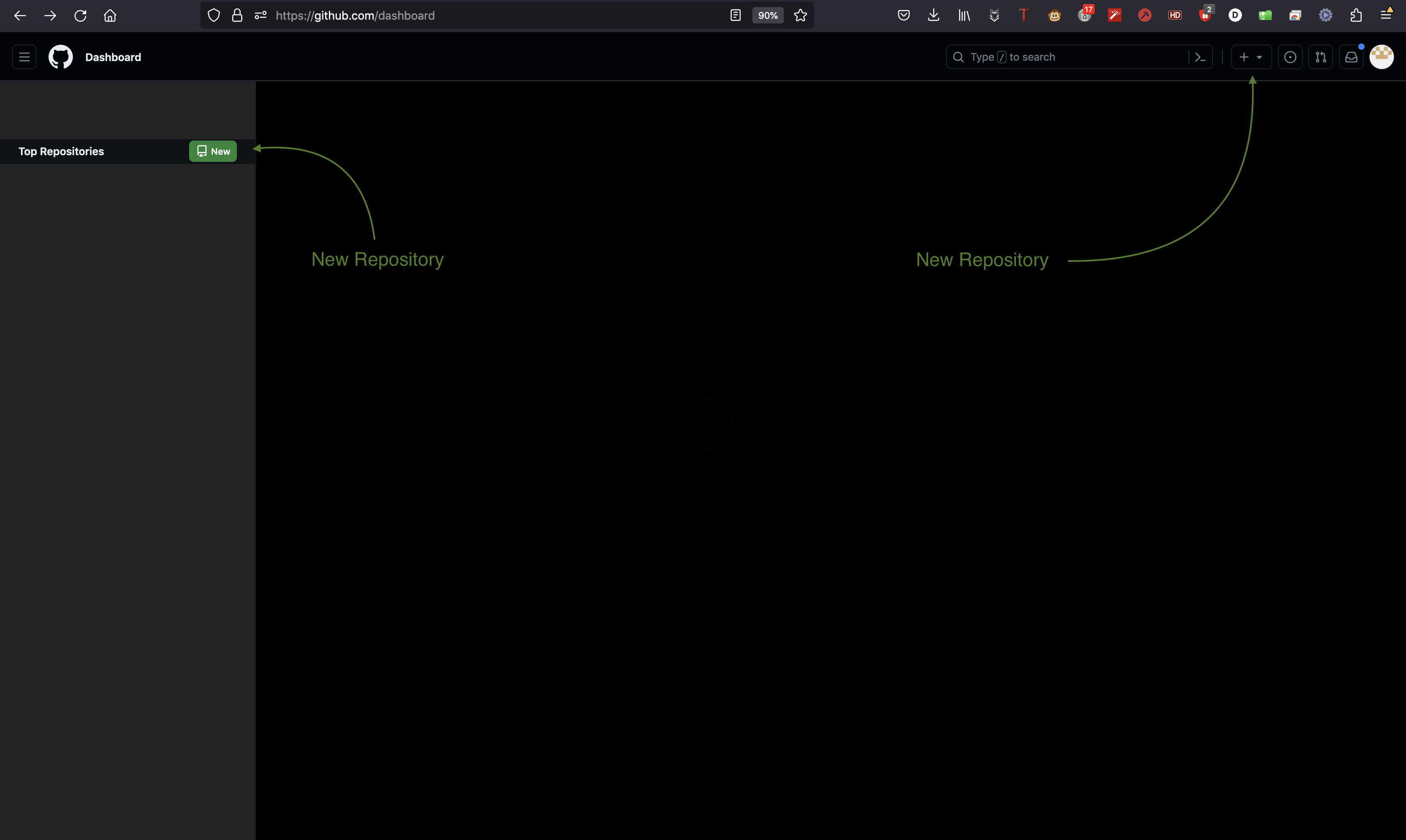
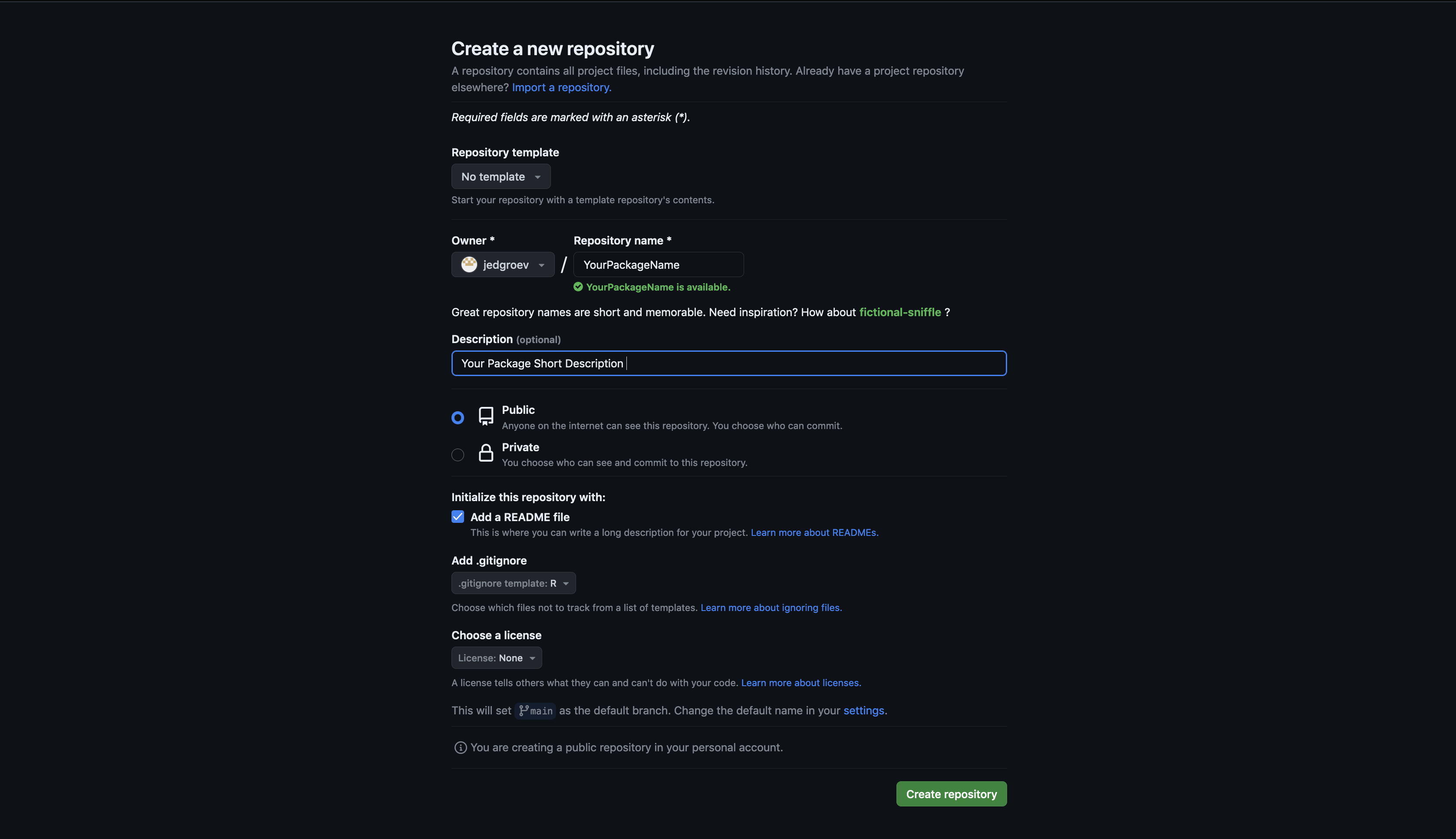
5.2. Create a new repository

Navigate to the GitHub or GitLab website and create a new project with a given name (YourPackageName). Include a README file during the initialization process and specify other optional settings (public/private, licensing, description).

New Repository Create Repository

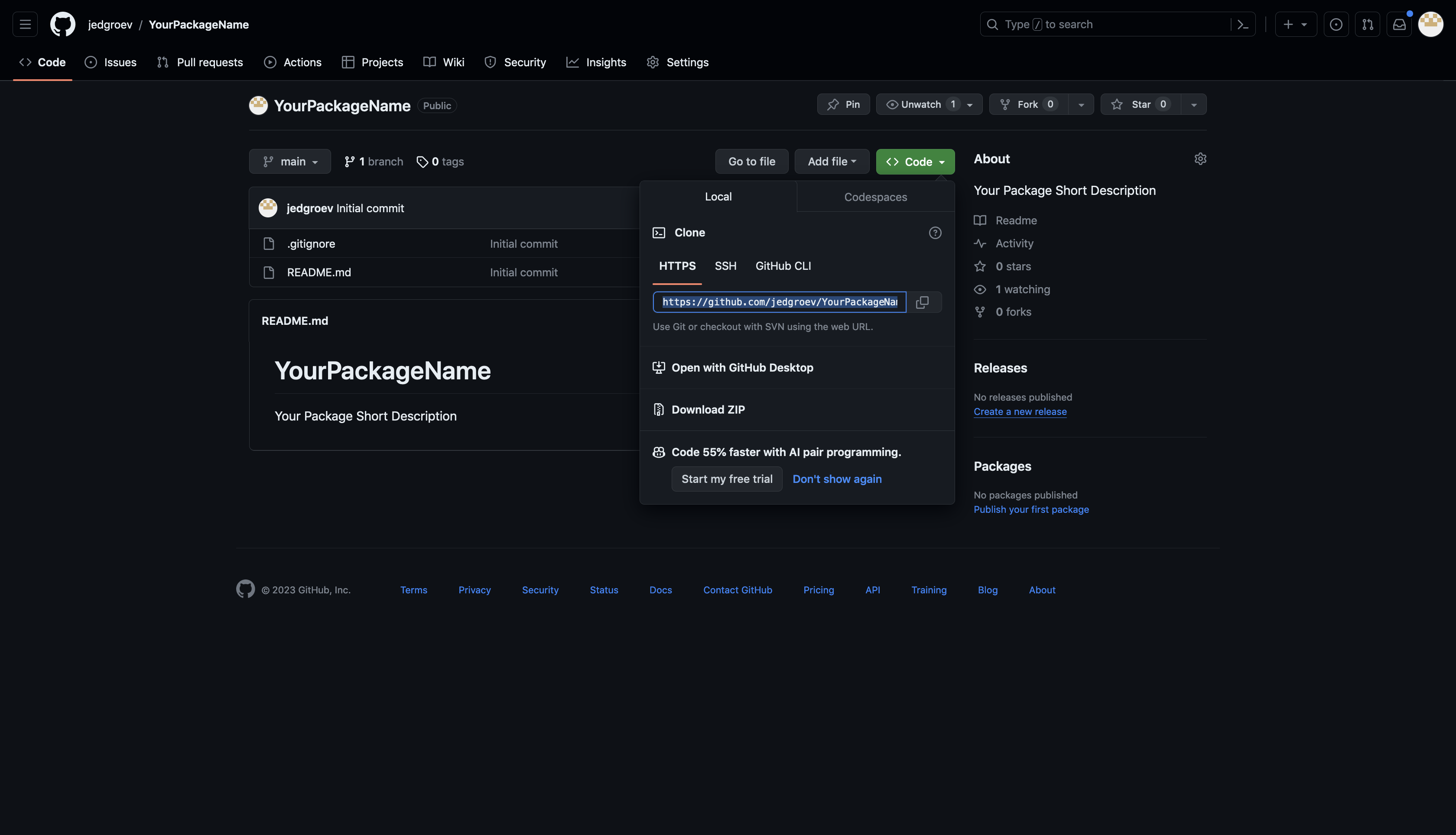
Copy repository link

Copy the HTTP link of your repository https://github.com/<YourAccount>/<YourPackageName>.git as shown in the figure below.

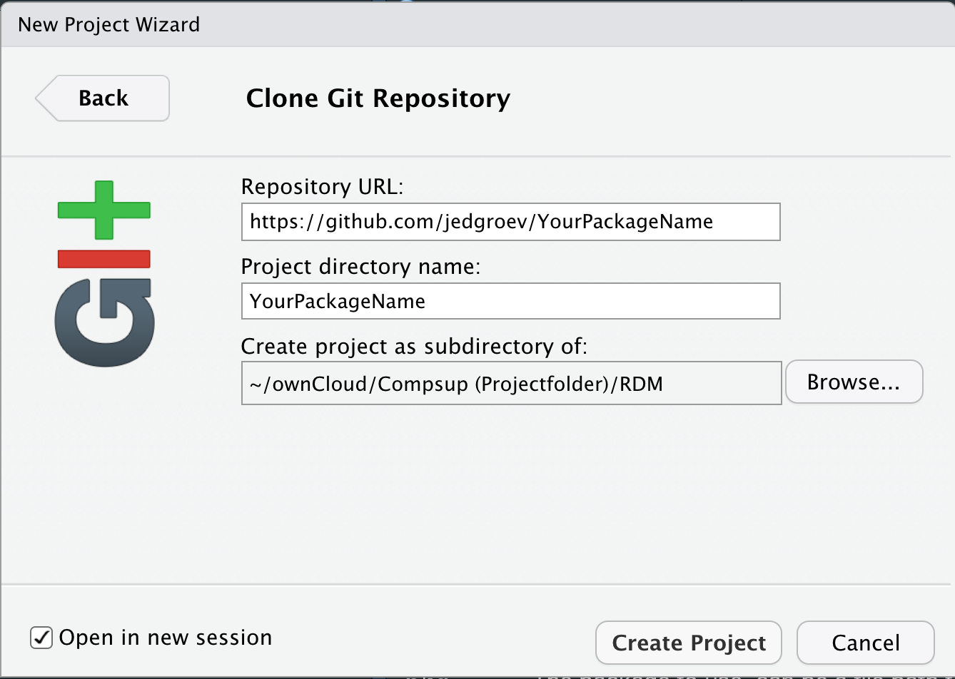
5.3. Set up repository in RStudio

Open RStudio and choose File -> New Project -> Version Control -> Git. Paste the Repository URL and specify the Project directory name (YourPackageName).

5.4. Modify gitignore file

Once you created a git project a file that is automatically created is the .gitignore in the root directory of your project. This is a file in which you can specify which files and directories that should be ignored and thus should not be versioned or hosted in Github or Gitlab.

Example .gitignore:

.Rhistory
.RData
data/input/

5.5. Make changes, commit and push

Once you have cloned the git repository you have the tools to version the files in your R package. To test this we can make changes into the README file and submit them to github/gitlab from within RStudio. There are several ways to submit changes in RStudio:

Use the shortcut command/ctrl + option/alt + M
Navigate to Tools -> Version Control -> Commit in the RStudio menu.
Navigate to the Git in upper-right panel in RStudio and click the Commit button.

A new window pops up in which you:

Select the files to which you want to add the specific commit message.
Add a message to describe the changes.
Click Commit to submit the changes to Git.
Click Push to push the committed changes to the git repository.

Git can also be used from the terminal:

git add <filename>
git commit -m "commit message"
git push <branchname>

NOTE: It is recommended to have pushed your changes by the end of the day, or when you stop working on a project. Before you start, the next day/moment/moment always make sure to first pull, to fetch changes made in GitHub or GitLab. Like that you ensure that both the online and local version remain synchronized.

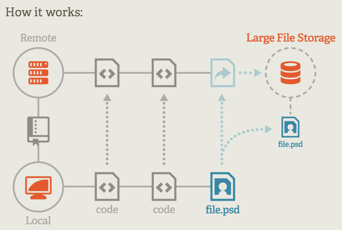
5.6 Git LFS

Large file support comes in handy if you would like to include large files in your package without bloating your git repository. Git Large File Storage (LFS) replaces large files such as audio samples, videos, datasets, and graphics with text pointers inside Git, while storing the file contents on a remote server like GitHub or Gitlab. To allow LFS navigate to https://git-lfs.com/ and download and install the extension.

5.6.1 Set up LFS

Once downloaded and installed, set up Git LFS for your user account by running:

git lfs install

You only need to run this once per user account.

5.6.2 Select file types

In each Git repository where you want to use Git LFS, select the file types you’d like Git LFS to manage.

git lfs track "*.html"

After running this a new file .gitattributes will be added to your repository including the file extensions that will be managed by LFS.

Example .gitattributes:

*.html filter=lfs diff=lfs merge=lfs -text

You can configure additional file extensions at anytime by running the above line of by directly editing .gitattributes.

git lfs track "*.zip"

Example .gitattributes:

*.html filter=lfs diff=lfs merge=lfs -text
*.zip filter=lfs diff=lfs merge=lfs -text

Exercise 5.1

Create a git repository named campaign2025 in github/gitlab.
Clone the repository locally.
Add all the content of the R-project created in previous exercises.
Commit and Push the changes.
Check your git-repository in github/gitlab.
Check the .gitignore file in the root of the directory and add data/input/.
Alternatively, instead of ignoring the images, you could also configure Large File Support (LFS). In that case, establish LFS and track .png files with LFS.
Open .gitattributes to see if .png is added.
Remove data/input/ from the .gitignore file.
Commit the changes to github.

6. Metadata

Documentation makes your project findable and reusable, two key FAIR principles, by providing metadata that describes the data consistently across a project and uniquely for individual datasets. Metadata can appear in a README (human-readable) or in a structured, machine-readable format (e.g., repository fields like title, creator, keywords, license), which enables indexing and discovery in catalogs and search engines. Well-structured metadata also supports accessibility by indicating how and where the data can be obtained, and interoperability by using shared standards and vocabularies, making it easier to combine and reuse datasets across projects.

We distinguish two levels of metadata: metadata that is consistent for all files in a project- and metadata that is unique for a dataset or file. The purpose of metadata is to provide sufficient information to reuse data and to use as much as possible metadata standards in doing that.

6.1 Project-level metadata

Project-level metadata often corresponds to metadata that needs to be provided when publishing a record in a general purpose repository (Zenodo, Figshare, Dryad). A good practice is to have all this metadata information available within a project-level README.md in the root directory.

The README should describe, the purpose of the project, folder structure, execution order of scripts. The README should also list the configurations that are needed to reproduce results of a project.

.
├── README.md
├── code/
├── data/
├── docs/
└── project_name.Rproj

Here is an example of a README for a data package including the persistent identifier of the publication to which it is linked, a directory tree and a description of both datasets and analysis scripts.

Other project-level metadata that could be added are CITATION and LICENSE. Both a citation and license file can be added in github.

6.1.1 License

Go to your repository on GitHub.

Click the “Add file” → “Create new file” button.
Name the file LICENSE (or LICENSE.txt).
GitHub will suggest popular licenses. You can click “Choose a license template” to select one (e.g., MIT, GPL-3.0, Apache 2.0).
GitHub will automatically fill in the license text. Fill in your name and year if required.
Scroll down and click “Commit new file” to add it to your repository.

6.1.2. Citation

A citation file makes it easy for others to cite your repository. GitHub recommends using a CITATION.cff file.

Go to your repository on GitHub.
Click “Add file” → “Create new file”.
Name the file CITATION.cff.
Add content using Citation File Format (CFF)

Exercise 6.1

Create a README.md for your project and add a description. Look at the example for inspiration.
commit the changes to the README.md to github.
Create a LICENSE file for your project in github.
Create a CITATION file in github.

6.2 Data-level metadata

A good practice for describing your dataset is to use the JSON format, and in particular the JSON-based metadata schema of the Frictionless Data standard. Via this app you can use an interface to enrich your dataset with metadata.

Frictionless metadata-template for tabular data

{
  "profile": "data-package",
  "resources": [
    {
      "name": "movement_data",
      "profile": "tabular-data-resource",
      "schema": {
        "fields": [
          {
            "name": "animal_id",
            "type": "integer",
            "format": "default",
            "description": "A unique numeric identifier for the animal",
            "title": "animal identifier"
          },
          {
            "name": "time",
            "type": "datetime",
            "format": "default",
            "title": "timestamp with time zone",
            "description": "Timestamp in UTC using the format YYYY-MM-DD hh:mm:ss"
          },
          {
            "name": "x",
            "type": "number",
            "format": "default",
            "title": "longitude",
            "description": "x-coordinate corresponds to longitude, using SRID 4326"
          },
          {
            "name": "y",
            "type": "string",
            "format": "default",
            "title": "latitude",
            "description": "y-coordinate corresponds to latitude, using SRID 4326"
          }
        ]
      },
      "title": "roe deer movement data",
      "description": "Roe deer (Capreolus capreolus) GPS movement data of five individuals from a North-Italian population monitored in 2025.",
      "path": "movement_data.csv"
    },
    {
      "name": "tree_cover_density_north_italy",
      "path": "tree_cover_density_north_italy.tif",
      "profile": "data-resource",
      "schema": {},
      "title": "Tree Cover Density 2021 - North Italy",
      "description": "Provides at pan-European level in the spatial resolution of 10 m the level of tree cover density in a range from 0% to100% for the 2021 reference year (SRID 3035).",
      "format": "tif",
      "encoding": "UTF8"
    }
  ],
  "keywords": [
    "roe deer",
    "Italy",
    "tree cover"
  ],
  "licenses": [
    {
      "name": "CC-BY-4.0",
      "title": "Creative Commons Attribution 4.0",
      "path": "https://creativecommons.org/licenses/by/4.0/"
    }
  ],
  "description": "Data package included movement data of five roe deer and tree cover density ",
  "name": "roe-deer-forest-cover-mapping",
  "title": "Roe deer forest cover mapping",
  "contributors": [
    {
      "title": "De Groeve, Johannes",
      "role": "author"
    }
  ]
}

Exercise 6.2

Use the frictionless app to create a metadata JSON for our input and output datasets:

01_species_observations

01_counts_per_species

01_counts_per_diet

img

solution

campaign2025

Exercise 6.3

Copy the file campaign2025 and save it in a JSON file named campaign2025.json in the root of your project directory.
Open the JSON file in your browser.
With which function would you load the JSON file in R?

solution

library(jsonlite)
library(dplyr)
library(tidyr)

# Parse JSON
json_data <- fromJSON('campaign2025.json', flatten = TRUE)

# Extract resources
resources <- json_data$resources

# Unnest while disambiguating field column names
resources_table <- resources %>%
  select(resource_name = name,
         resource_title = title,
         resource_description = description,
         path,
         schema.fields) %>%
  unnest(schema.fields, names_sep = "_", keep_empty = TRUE)

resources_table

7. Project Dependency Management with `renv`

renv is an R package that helps manage project-specific dependencies, ensuring reproducibility across different environments. It creates an isolated library for each project, allowing you to install and use package versions that won’t conflict with other projects or your system-wide R setup. You can record the exact packages and versions used in a project with renv::snapshot() and later restore them on the same or another machine using renv::restore(), ensuring consistent behavior. For example, to initialize a project with renv, you can run:

# Initialize renv for the project
renv::init()

# Install a package
renv::install("dplyr")

# Record the current package versions
renv::snapshot()

When using renv with Git, the .gitignore file should exclude the project library (renv/library/) to avoid tracking large or machine-specific files. Typically, the renv.lock file is included in version control since it defines the exact package versions for reproducibility.

Example .gitignore:

.Rhistory
.RData
renv/library

To make it easier to detect and install dependencies used in your scripts, you can create a dependencies.R file in the project root that scans your R code for package usage:

# file: dependencies.R
if (FALSE) {
library(dplyr)
}

This way, any collaborator can quickly install all required packages for a specific script before running the analysis, while renv::restore() ensures the full project environment is reproducible.

For an example:

Exercise 7.1

Setup an R environment for your project and include all the useful R packages (tidyverse, terra, stars, mapview, mapedit, move2, amt, knitr, data.table, lubridate, targets) mentioned in section 3.5.
Add renv/library to the .gitignore file.
Commit the changes to github.
Run once more the function fs::dir_tree(recurse=4) to obtain the directory tree up to a depth of 4 directories.

solution

renv::init()

renv::install(c("tidyverse", 
                "terra", 
                "stars", 
                "mapview", 
                "mapedit", 
                "move2", 
                "amt", 
                "knitr", 
                "data.table", 
                "lubridate", 
                "targets"))

renv::snapshot()

Wrap-Up

Through this tutorial, you have practiced building a fully structured, reproducible, and FAIR-aligned R project. By applying consistent file formats, folder structures, metadata, version control, and open tools, your project becomes easier to share, reproduce, and build upon—core to modern scientific collaboration.

As you transition to real-world projects, revisit these principles often. The goal is not just organization but building research workflows that support scientific integrity, trust, and collaboration.

Introduction

1. Directory structure and file naming

1.1 Directory structure

1.1.1 Informed, simple, structured and consistent

Exercise 1.1

1.1.1 Case study: Camera trapping images

1.1.1.1 Main data directory

1.1.1.2 Subdirectories

1.1.2 R Projects

Exercise 1.2

Exercise 1.3

1.2 File naming

1.2.1 Metadata is key

1.2.2 Case study: Camera trapping images

1.2.3 General file naming rules

1.2.3.1 Computer-readable file names

1.2.2.2 Human-readable file names

1.2.2.3 File names that work well with default ordering

Exercise 1.4

1.3. Tips for Good File and Directory Organization

2. Spreadsheets

2.1 What are spreadsheets good for?

2.2 Human-readable vs. computer-readable data

2.3 Tidy data

2.4 Problematic practices

2.4.1 Multiple variables in a single column

2.4.2 Rows for variables, columns for observation

2.4.3 Multiple tables in a single spreadsheet

2.4.4 Multiple sheets

2.4.5 Using formatting to convey information

2.4.6 Putting units in cells

2.4.7 Using problematic column names

2.4.8 Conflating zeros and missing values

2.4.9 Using problematic null values

2.4.9.1 Inconsistent value formatting

2.5 Document

Exercise 2.1

3. Code Management

3.1. Comment your code

3.2. Use a style guide

3.3. Functions

3.4. Quarto (.qmd)

3.5. Useful R Packages

3.6 Tips for Code Management

Exercise 3.1

Exercise 3.2

4. File Formats

5. Git

5.1. Setting Up Git in RStudio

5.2. Create a new repository

Copy repository link

5.3. Set up repository in RStudio

5.4. Modify gitignore file

5.5. Make changes, commit and push

5.6 Git LFS

5.6.1 Set up LFS

5.6.2 Select file types

Exercise 5.1

6. Metadata

6.1 Project-level metadata

6.1.1 License

6.1.2. Citation

Exercise 6.1

6.2 Data-level metadata

Exercise 6.2

7. Project Dependency Management with renv

Exercise 7.1

Wrap-Up

7. Project Dependency Management with `renv`